
Coherence theory is the study of correlations that exist between different parts of a light field. Temporal coherence indicates a correlation between fields offset in time, E(r,t) and E(r,t − τ). Spatial coherence has to do with correlations between fields at different spatial locations, E(r,t) and E(r + ∆r,t). Because light oscillations are too fast to resolve directly, we usually need to study optical coherence using interference techniques. In these techniques, light from different times or places in the light field is brought together at a detection point.
If the two fields have a high degree of coherence, they consistently interfere either constructively or destructively at the detection point. If the two fields are not coherent, the interference at the detection point rapidly fluctuates between constructive and destructive interference, so that a time-averaged signal does not show interference. You are probably already familiar with two instruments that measure coherence: the Michelson interferometer, which measures temporal coherence, and Young’s two-slit interferometer, which measures spatial coherence.
Your preliminary understanding of these instruments was probably gained in terms of single-frequency plane waves, which are perfectly coherent for all separations in time and space. In this chapter, we build on that foundation and derive descriptions that are appropriate when light with imperfect coherence is sent through these instruments. We also discuss a practical application known as Fourier spectroscopy (Section 8.4) which allows us to measure the spectrum of light using a Michelson interferometer rather than a grating spectrometer.
Michelson Interferometer
A Michelson interferometer employs a 50:50 beam splitter to divide an initial beam into two identical beams and then delays one beam with respect to the other before bringing them back together. Depending on the relative path difference d (roundtrip by our convention) between the two arms of the system, the light can interfere constructively or destructively in the direction of the detector.
Coherence Time and Fringe Visibility
The coherence time τc is the amount of delay necessary to cause γ(τ) to quit oscillating (i.e. its amplitude approaches zero). This definition is not very precise, since the oscillations do not usually have an abrupt end, but instead slowly die off as τ increases. A useful (although arbitrary) analytic definition for the coherence time
Consider a continuous light source such as starlight or a continuous wave (CW) laser. The integral R ∞ −∞ I(t)d t diverges for such a source since it is on forever (or at least for a very long time) and emits infinite (or very much) total energy. The concept of fluency (i.e. total energy) in this case is not very useful. However, note that the integrals on both sides of (8.5) diverge in the same way. We can renormalize (8.5) in this case by replacing the integrals on each side with the average value of the intensity
Although technically the integrals used in (8.10) to compute γ(τ) also diverge in the case of continuous light, the numerator and the denominator diverge in the same way. Therefore, we may renormalize I (ω) in a similar fashion to deal with this problem. The units in the numerator and denominator cancel so that γ(τ) always remains dimensionless. Once we have the degree of coherence function γ(τ), we can calculate the coherence time and fringe visibility just as we did for pulsed sources.
Fourier Spectroscopy
The Fourier transform of the measured signal is seen to contain three terms, one of which is the power spectrum I (ω) that we are after. Fortunately, when graphed as a function of ω (shown in Fig. 8.5), the three pieces on the right-hand side of (8.20) do not overlap. As a reminder, the measured signal as a function of τ looks like something.
Making an informed decision is crucial when considering Vidmate old version. Benefits include familiarity and stability. Drawbacks may involve security risks and lack of updates. Evaluate your needs carefully before choosing. Ensure compatibility with your device and consider potential risks. Ultimately, the decision rests on your priorities. Balance the advantages and disadvantages to make the best choice.
Last word
The oscillation frequency of the fringes lies in the neighborhood of ω0. In summary, to obtain I (ω) using a Michelson interferometer, 1) record Sig(τ); 2) take its Fourier transform; and 3) extract the curve at positive frequencies.